Sparse Merkle Tree vs Indexed Merkle Tree

[kd14]

Nullifiers are cryptographic markers derived from spent notes, used to prevent double-spending in privacy-preserving systems. Once revealed, nullifiers become public information. In traditional systems, nullifiers are stored in sets maintained locally by validators. However, this approach requires validators to maintain the full nullifier set state, which can become costly and inefficient over time.

This document introduces a compact data structure, known as a nullifier tree, which eliminates the need for validators to store the nullifier set state. Instead, validators verify operations on the nullifier tree to ensure that nullifiers are correctly managed. Nullifier trees enable efficient verification of whether a nullifier has already been spent, while significantly reducing the storage and computational overhead for validators. This approach ensures data integrity and facilitates fast and secure transaction validation without compromising scalability

This document compares two primary data structures for implementing nullifier trees in Nomos:

• Sparse Merkle Trees (SMTs)
• Indexed Merkle Trees (IMTs)

The objective is to evaluate these structures based on performance, scalability, and implementation complexity to determine their suitability for the Nomos ledger protocol.

Overview

This document provides a technical comparison between Sparse Merkle Trees (SMTs) and Indexed Merkle Trees (IMTs) in the context of implementing nullifier trees for the Nomos ledger protocol. The goal is to evaluate both structures based on:

• Performance: Time and computational complexity.
• Scalability: Handling large nullifier sets.
• Implementation Complexity: Ease or difficulty of integration, especially for zero-knowledge circuits.

In the document, SMT and IMT structures have been examined separately, and their features have been explained. Then, the differences between the two structures and performance comparisons have been made. Additionally, the details of the implementations performed for SMT and IMT have also been shared. As a result of the studies conducted, it has been observed that the IMT structure provided better performance results for Nomos ledger representation. Moreover, to achieve an efficient implementation, the IMT structure was slightly modified and used together with a Merkle Mountain Range (MMR). The details of this custom usage are explained in the relevant section

The following sections delve into the initialization, update, and proof processes for each data structure, highlighting their ZK circuit complexity, storage requirements, and performance characteristics.

Sparse Merkle Tree (SMT)

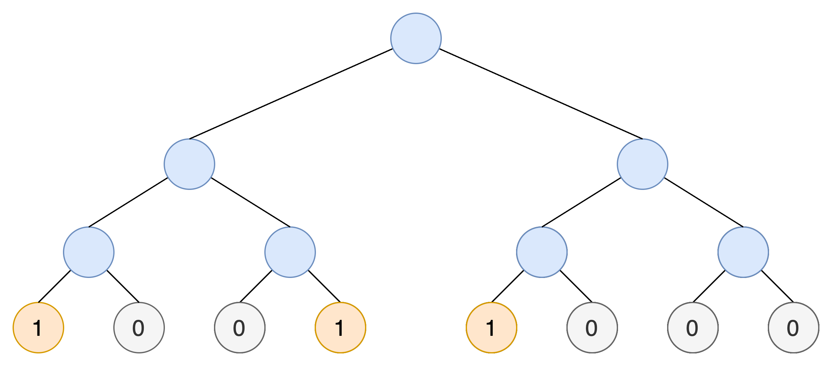
A Sparse Merkle Tree is a cryptographic data structure designed to store data in a way that allows for efficient verification of data existence or non-existence. It is characterized by having a fixed size, determined by the number of possible elements in the set, which creates a vast number of leaves. Each leaf corresponds to a potential index in the tree, derived by hashing an element of the set, and is initially initialized to a default value, representing the absence of any element at that position. When a value is added to the tree, the corresponding leaf is updated to reflect its inclusion, and the hashes along the path to the root are recomputed to maintain the tree’s integrity.

SMTs are designed to handle large namespaces without requiring explicit storage of all leaves. Instead, only non-empty leaves and the hashes along their paths are stored explicitly, while empty leaves are represented implicitly using a default value (0 or a fixed hash).

Initialization Process

1. Tree Structure:
   • An SMT represents an updatable tree where each nullifier nf directly maps to a pre-determined index in the tree. When using an SMT for nullifiers, deletion is not supported, as nullifiers are designed to remain in the tree once added to prevent double-spending.
   • The tree size is defined by the largest possible nf. For example, for 256-bit nullifiers, the tree requires 2^{256} leaves, though sparsely populated.
2. Default Values:
   • All leaves are initialized with a default value 0, representing the absence of data.
3. Recursive Hashing:
   • Internal nodes are recursively computed from leaf hashes to the root, ensuring the tree structure is valid.
   • This is possible because for each layer in the tree, every node has the same children and then the same value.

Algorithm:

def initialize_smt(depth):
	# Initialize the deepest layer to 0 to represent that there is no value.
	root = 0
	for i in range(depth):
		root = hash(root, root)
	return root

Update Process

1. Direct Mapping:
   • The nullifier nf determines the index of the leaf directly (e.g., nf=5 updates the 5th leaf).
2. Update Leaf Value:
   • Update the leaf value at index to 1 to represent the presence of nf.
3. Recompute Path:
   • Recompute hashes along the path from the updated leaf to the root.

Algorithm:

def update_smt(tree, nf):
    index = nf  # Nullifier directly determines the index in SMT
    tree.leaves[index] = 1  # Mark presence of the nullifier with value 1

    # Recompute hashes along the path from the leaf to the root
    recompute_hashes(tree, index)

def recompute_hashes(tree, index):
    """
    Recompute hashes from the updated leaf to the root of the tree.
    :param tree: Sparse Merkle Tree data structure
    :param index: Index of the updated leaf
    """
    current_index = index
    current_value = tree.leaves[current_index]  # Leaf value is 1 
    for level in range(tree.depth):
        sibling_index = current_index ^ 1 
        sibling_value = tree.nodes[level].get(sibling_index, 0)  
        parent_index = current_index // 2
        tree.nodes[level + 1][parent_index] = hash(
            str(current_value), str(sibling_value)
        )

        # Move up the tree
        current_index = parent_index
        current_value = tree.nodes[level + 1][parent_index]

Algorithm for SMT Batch Update

In SMTs, batch updates are achieved by updating multiple leaves in the tree simultaneously. Each nullifier corresponds to a fixed index (determined by hashing the nullifier), and updates proceed as follows:

1. Identify Indices:
   • Compute the indices for all nullifiers by hashing their values.
   • For example: index_1 = H(nullifier_1), index_2 = H(nullifier_2).
2. Group Updates:
   • Identify overlapping paths in the tree.
   • For example, if two nullifiers are close to each other in the tree, their paths to the root will share common nodes.
3. Compute Updates:
   • Update the leaves at the computed indices.
   • Recompute hashes for each path to the root, reusing computations for shared paths.

Non-Membership Proof

1. Generate Proof:

   • For a nullifier nf, retrieve the Merkle proof path for the leaf at index nf.

   To generate the proof, the algorithm iterates from the leaf node (at index nf ) up to the root, retrieving the sibling hash at each level.

   • Include the flag value 0 (indicating absence) from the leaf.

2. Verify Proof:

   • Using the proof path, verify that the flag value 0 correctly reconstructs the root, confirming that no nullifier exists at index nf.

Algorithm:

def generate_non_membership_proof_smt(tree, nf):
    """
    Generate a Merkle proof for non-membership in an SMT.
    Args:
        tree: Sparse Merkle Tree.
        nf: Nullifier (used as index).
    Returns:
        proof_path: The Merkle proof path for the leaf.
    """
    proof_path = get_merkle_path(tree, nf)  # Retrieve Merkle path for index nf
    return proof_path

def verify_non_membership_proof_smt(root, proof_path, nf):
    """
    Verify a non-membership proof in an SMT.
    Args:
        root: Root of the Merkle Tree.
        proof_path: Merkle proof path.
        nf: Nullifier (used as index).
    Returns:
        True if the proof is valid, False otherwise.
    """
    # Reconstruct the root using the Merkle proof and the default flag value (0)
    leaf_value = 0  # Non-membership implies the leaf value is 0
    computed_root = compute_root_from_proof(proof_path, nf, leaf_value)
    return computed_root == root

Properties of SMTs

• Non-membership proofs are inherent to the structure, as leaves representing non-membership are initialized to a default value that can be verified directly, without requiring extra data or checks compared to proving membership.
• Proof size is constant, determined by the fixed depth of the tree, which relies on the maximum possible size of the set, making it predictable and scalable.
• Executors only need to store the non-empty leaves and internal nodes on the path (required to reconstruct the path from any non-empty leaf to the root), which minimizes memory usage.
• ZK circuit complexity in SMTs is influenced by the fixed tree depth, which requires 256 hashes for proofs (for Nomos’ nullifiers). While predictable and consistent, non-membership proofs in SMTs may require more computation compared to IMTs for smaller datasets due to the larger number of hashes needed to point to the correct location.
• Inefficient for systems with a smaller number of nullifiers, as the tree height is determined by the maximum possible set size, not the current number of nullifiers.

Indexed Merkle Tree (IMT)

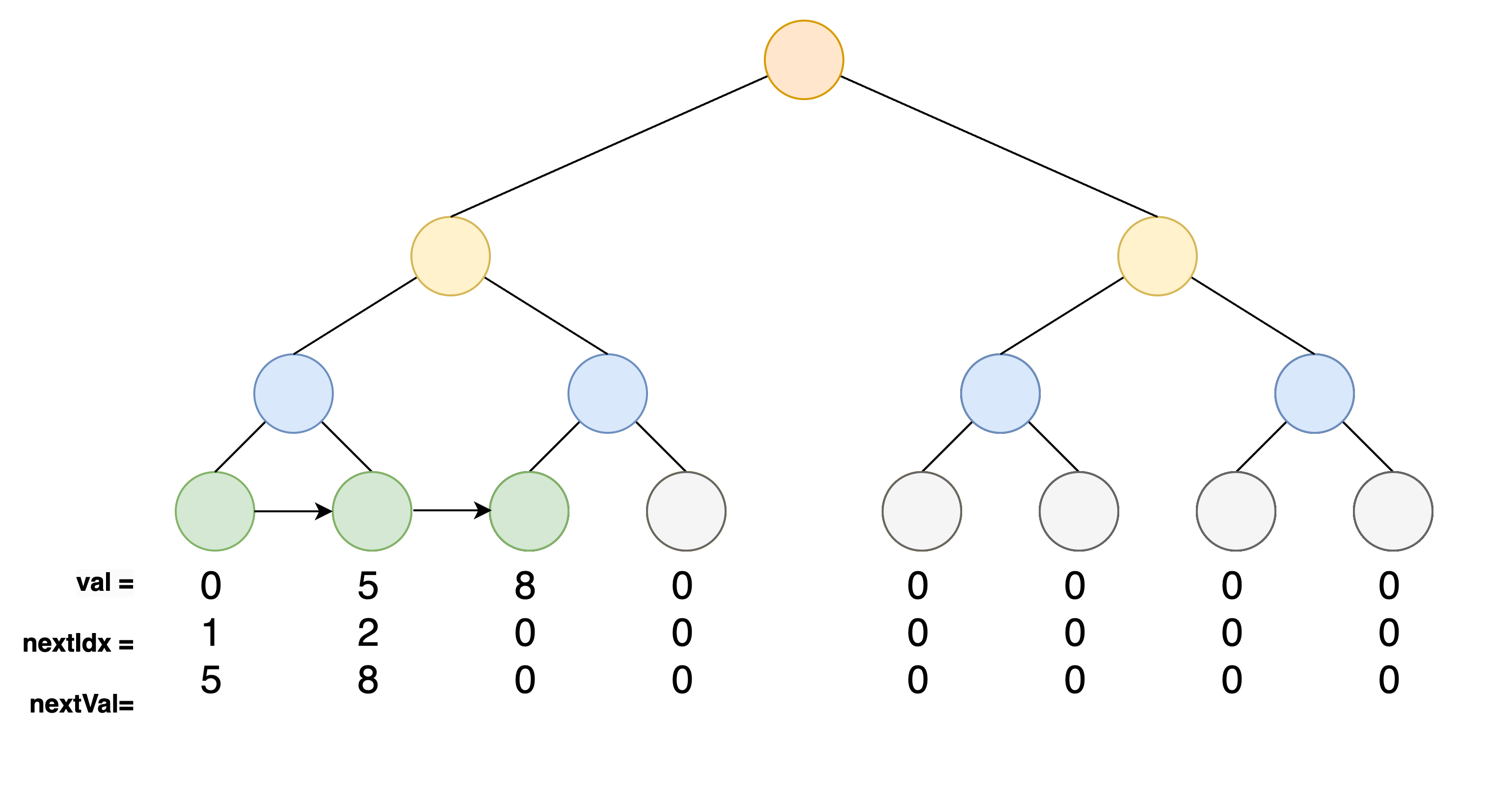
An Indexed Merkle Tree, on the other hand, enhances the SMT by explicitly linking nullifiers in a sorted linked list structure within the tree, where each leaf contains the next nullifier value and may also include the index of the next leaf, enabling efficient range and adjacency checks. This innovation allows for not only efficient proof of existence but also streamlined batch operations and non-inclusion proofs. In an IMT, value of the leaves are sorted, and each node maintains a pointer to its successor, enabling the tree to grow dynamically while reducing computational overhead for operations such as range checks or batch insertions.

Initialization Process

1. Empty Tree:
   • Start with an empty root and no leaves.
2. Initial Leaf:
   • Optionally prepopulate the tree with a “sentinel” leaf at index 0 with v=0, i_\text{next} = 0, v_\text{next} = 0.

Algorithm:

def initialize_imt():
    sentinel_leaf = {"v": 0, "i_next": 0, "v_next": 0}  # Sentinel leaf
    return {"root": None, "leaves": [sentinel_leaf]}  # Initialize with sentinel

Update Process

Steps:

1. Find Position:
   • Determine the correct position for nf by iterating through the sorted leaves.
   • Identify i_\text{lower}, the index of the preceding leaf, such that v_\text{lower} < nf < v_\text{next(lower)}.
2. Create New Leaf:
   • Construct the new leaf \{v = nf, i_\text{next} = i_\text{next(lower)}, v_\text{next} = v_\text{next(lower)}\}.
3. Update Adjacency:
   • Update i_\text{next} and v_\text{next} fields of the preceding leaf:
     • i_\text{next(lower)} = \text{index of the new leaf}
     • v_\text{next(lower)} = nf
4. Recompute Merkle Path:
   • Update the hashes along the path to the root to maintain tree consistency.

Algorithm:

def update_imt(tree, nf):
    # Step 1: Create new leaf
    new_leaf = {
        "v": nf,
        "i_next": lower_leaf["i_next"],
        "v_next": lower_leaf["v_next"]
    }

    # Step 2: Update adjacency pointers of the lower leaf
    lower_leaf["i_next"] = len(tree.leaves)
    lower_leaf["v_next"] = nf

    # Step 3: Insert the new leaf
    tree.leaves.append(new_leaf)

    # Step 4: Recompute Merkle path
    recompute_hashes(tree, lower_index)

Algorithm for IMT Batch Update

IMTs handle batch updates more efficiently by leveraging adjacency pointers. Instead of independently updating each nullifier, the algorithm finds the range of nullifiers affected and updates the structure in a grouped operation.

Summary of the Protocol

1. Sort Nullifiers:
   • Ensure the batch of nullifiers is sorted: {N1, N2, N3, ...}.
2. Determine Adjacency:
   • For each nullifier, find its predecessor (prev) and successor (next) determining where it falls between two nullifiers that are either in the batch or in the IMT.
   • For example, N2 is inserted between N1 and N3 if there is no nullifier closer to N2 in the IMT.
3. Update Pointers:
   • Update the next pointer of prev to point to the new nullifier.
   • Update the next pointer of the new nullifier to point to next.
4. Insert Nullifiers:
   • Add the new nullifiers to the tree.
   • Recompute hashes for all affected paths to the root. During batch insertion, the new nullifiers are added to the tree as a sub-tree in an internally sorted order. In this case, the sub-tree affects all parent nodes up to the root from the point where it is added. In this case, just like with a normal insertion, the value of the lowest nullifier in the main tree and the closest node value in the added subtree will be updated.

Deterministic Insertion: Since nullifiers are inserted deterministically, entire subtrees can be inserted rather than appending nodes individually.

Subtree Insertion: We first prove that the subtree we’re inserting consists of all empty values. This is done by performing an inclusion proof for an empty root, proving that there is nothing within the subtree.

Re-create Subtree: The subtree is recreated within the circuit, and the new root is computed after inserting the subtree.

Update Pointers: During insertion, we must update the low nullifier pointers to ensure the tree maintains its structure.

Non-Membership Proof Generation

This is the witness generation step, which produces the proof for non-membership.

To prove that a nullifier nf does not exist in the IMT:

1. Retrieve the Merkle proof path for the predecessor nullifier leaf (v_lower), where v_lower is the maximum value in the set smaller than nf.
2. Use the adjacency property to show that v_lower < nf < v_next, where v_next is the next nullifier value in the predecessor leaf.

Protocol Steps

1. Find Predecessor Leaf:
   • Locate i_\text{lower}, the index of the preceding leaf, where v_\text{lower} is the maximum nullifier smaller than nf.
2. Generate Witness:
   • Retrieve the Merkle proof path for i_\text{lower}.
   • Include the predecessor leaf {v_\text{lower}, i_\text{next(lower)}, v_\text{next(lower)}} as the witness.

Algorithm:

def generate_non_membership_proof_imt(tree, nf):
    # Step 1: Find predecessor leaf (witness generation)
    lower_index = find_predecessor(tree.leaves, nf)
    lower_leaf = tree.leaves[lower_index]

    # Step 2: Generate Merkle proof for lower leaf
    proof_path = get_merkle_path(tree, lower_index)

    return proof_path, lower_leaf  # Return proof path and witness

Non-Membership Proof Verification

This step verifies the proof generated using the witness.

To verify the non-membership proof:

1. Confirm the adjacency relationship using the witness (v_lower): v_\text{lower} < nf < v_\text{next(lower)}.
2. Validate the Merkle proof path to ensure the leaf correctly reconstructs the root.

Protocol Steps:

1. Verify Adjacency:
   • Perform a range check: v_\text{lower} < nf < v_\text{next(lower)}.
2. Merkle Root Validation:
   • Use the proof path and witness to compute the Merkle root.
   • Verify that the computed root matches the expected root.

Algorithm:

def verify_non_membership_proof_imt(root, proof_path, lower_leaf, nf):
    # Step 1: Verify adjacency (range check)
    if not (lower_leaf["v"] < nf < lower_leaf["v_next"]):
        return False

    # Step 2: Verify Merkle root using witness
    computed_root = compute_root_from_proof(proof_path, lower_leaf)
    return computed_root == root

• How Updates Work in IMTs:

  • Once a nullifier is added to a leaf, it remains in that position. The value of the leaf does not move or change location within the tree.
  • Adjacency pointers (linking a nullifier to the next higher nullifier) are the components that need updating when a new nullifier is added.
    • For example, when a new nullifier is falling in the range of two existing nullifiers, the pointers of the predecessor leaf in the sorted list is updated to link the new nullifier correctly.
  • After the new nullifier is added, the hashes along the path from the updated leaf to the root are recomputed to maintain the integrity of the Merkle tree. This operation has a complexity of O(\log n), where n is the number of leaves in the tree.
  • Since leaf values remain static, non-membership proofs become more efficient. The system can prove a nullifier’s absence by providing:
    1. A Merkle proof for the lower (predecessor) nullifier, which contains the actual value and the next nullifier value.
    2. A range check showing that the nullifier in question lies between the predecessor and its successor (if it exists). This is just a simple check, no need any proof verification.
  • This adjacency-based approach simplifies non-membership proofs by focusing only on the relationship between a nullifier and its adjacent nullifiers.

  Note
  Circom does not support dynamic tree sizes due to its reliance on static constraints and fixed circuit structures. This limitation makes implementing an IMTs more challenging compared to platforms like Risc0, which are more flexible in terms of dynamic data structures.

  To account for Circom’s fixed-depth requirement:

  • Set the tree depth D to a value that accommodates the expected maximum number of nullifiers.
  • Use sentinel nodes to fill unused portions of the tree.

Properties

• Compact and efficient for smaller datasets, as the tree grows dynamically with the number of nullifiers: IMTs are particularly well-suited for smaller datasets, where the number of nullifiers isn’t very large—a scenario that is often practical in real-world applications. Unlike SMTs, which operate within a fixed 256-bit namespace regardless of the dataset size, IMTs grow dynamically with the number of active nullifiers. This dynamic structure eliminates the inefficiencies of managing a vast, sparsely populated tree, making IMTs a more efficient and compact choice for systems with smaller nullifier sets.
• Non-membership proofs are possible by showing adjacency (i.e., proving a nullifier is between two others) which requires only one Merkle proof and two comparisons.
• IMTs offer smaller ZK circuits for proof verification due to their reduced depth, though the additional complexity of maintaining ordered pointers can increase insertion proof costs during batch insertions, making the overall ZK circuit size context-dependent. IMTs offer smaller ZK circuits for proof verification due to their reduced depth (e.g., 64 levels), requiring fewer hashes compared to SMTs. However, during batch insertions, the circuit must verify adjacency and update pointers for each nullifier, increasing the ZK circuit size proportionally to the batch size.
• Flexible for incremental systems or during the initial phases of deployment.
• Non-membership proofs are more complex because the tree depth is variable, and the proof involves comparisons rather than simple equality checks.
• Executors need to manage sorting outside the circuit, which ensures nullifiers are in a sorted order. Inside the circuit, updates involve only two comparisons (for the predecessor and successor values) and recomputation of the affected Merkle path.

Comparison Summary (up to 2^{64} nullifiers)

Aspect	SMT	IMT
Non-Membership Proof Complexity	Fixed-size proof; 256-depth Merkle proof and 1 equality check.	Single 64-depth Merkle proof, 2 comparisons, and verification of adjacency pointers.
ZK Circuit Complexity	Higher: 512 hashes per proof + 1 equality comparison.	Lower: 192 hashes + 2 comparisons per proof.
Storage Requirements	Compact for executors, as only non-empty leaves and their Merkle paths are stored. (Merkle paths may need to be recomputed on demand to save storage.)	Additional space is needed for storing pointers at each node. However, this overhead is manageable since executors typically maintain nullifiers in a sorted list to avoid rescanning the entire tree.
Implementation Complexity	Simpler to manage as it avoids dynamic pointer allocation and updates existing pre-initialized leaves over time.	More complex due to pointer management and dynamic structure.
Flexibility	Limited by static structure and predetermined depth.	More adaptable due to dynamic depth and efficient updates.
Insertion Overhead	Straightforward append-only mechanism.	Involves updating pointers and modifying existing leaves, which can be efficiently executed, potentially making it faster.

Conclusion

Sparse Merkle Tree

Advantages:

• Simpler to implement due to its lack of dynamic pointer management and reliance on updating pre-initialized leaves.
• Constant proof size and predictable performance make it ideal for systems with steady nullifier growth and fixed-depth requirements.

Disadvantages:

• Requires significantly more computational effort for proofs due to its fixed-depth structure (e.g., 512 hashes for a 256-depth tree).
• Inefficient for moderate nullifier growth or dynamic scenarios.

Indexed Merkle Tree

Advantages:

• More efficient for moderate datasets, as its dynamic depth significantly reduces the number of hashes required for proofs (e.g., 192 hashes for a 64-depth tree).
• Compact and efficient proofs due to adjacency pointers and reduced tree depth.
• More flexible and better suited for systems requiring efficient updates or batch insertions.

Disadvantages:

• Insertion involves pointer updates and potential leaf modifications, adding to implementation complexity.

Key Trade-Offs

• SMT: Prioritizes simplicity and predictable performance at the cost of higher proof computation. Best for large-scale systems requiring scalability with minimal implementation complexity.
• IMT: Offers superior proof efficiency and adaptability, but requires careful consideration of pointer management and increased memory usage. Best for systems with moderate nullifier sets and dynamic requirements.

Given the updated understanding of proof efficiency, Indexed Merkle Trees outperform Sparse Merkle Trees in terms of computational efficiency and proof size when managing moderate datasets (2^{64} nullifiers).

Sparse Merkle Tree vs. Indexed Merkle Tree in Terms of Batch Insertion

• Sparse Merkle Tree:
  • Sparse trees require a depth proportional to the size of the elements, which means that batch insertions are less efficient due to the need to perform many hashes for each insertion.
  • Inserting multiple nodes requires sequential updates, making it computationally expensive.
• Indexed Merkle Tree:
  • Indexed trees allow for more efficient batch insertions compared to SMT. The structure is more like a linked list, allowing for batch updates with fewer constraints.
  • Batch insertions can be done by inserting subtrees, significantly reducing the number of operations needed compared to sparse trees.

IMT with MMR Structure

IMT updates as described above only work when the tree has available empty space for new value insertions. If the tree is full (for example, when it starts small), you must grow the tree to create that free space. In this context, we refer to the frontier nodes of the MMR as the minimal set of nodes needed to continue expanding the structureThis requires showing that the new root—where you’ll prove membership of the empty subtree—can be obtained by merging the old tree with an empty tree of equal size, increasing the tree depth by 1.

Additionally, when inserting a variable number of values, they may not all fall within a single contiguous full subtree, forcing you to divide the batch into multiple sub-batches.

To address both challenges, we enhance the IMT with a supplementary data structure used exclusively during updates. All other operations remain unchanged and fully compatible with this modification.

Batch Update

We will focus on batch updates, as they are most relevant to our needs. Note that a single update is simply a batch of size 1.

• Non-membership: The update begins by proving non-membership of the values to be added. This is accomplished by providing a membership proof of the previous nullifier in the tree, as described above.
• Update of low nullifiers: Next, we update existing tree values (the predecessors of values being added) to reflect the updated pointers. For example, if the tree contains leaf l {value: 100, next: 110} and we want to add nullifier 105, we must update the next field of l to l': {value: 100, next: 105}. Using the merkle path that proves membership of l, we can compute the root with l' instead of l to demonstrate that only this value was modified. After this, we still need to add the new nullifiers to the tree.When updating multiple existing leaves, proving correct updates becomes more complex because after the first update, the membership proofs of other leaves become outdated. To handle this, we process updates sequentially. Only the first merkle path needs to be constructed relative to the original tree—subsequent membership paths for low nullifiers will be relative to the tree after each previous update.For example, starting with root r and needing to modify leaves l1 and l2:
  • First, we show that there’s a valid merkle path from l1 to r
  • Then we update the next field of l1 and calculate the new root r' using the same path.
  • Next, we show that there’s a valid merkle path from l2 to r' (not r!).
  • Then, we update next field of l2 and calculate the new root r'' using the same path.
  • …repeat the process if there are more leaves to update
• Add new nullifiers: This step introduces the most significant changes. Rather than proving the existence of empty subtrees, we demonstrate knowledge of the tree’s frontier—a list of complete subtrees within the tree. The frontier list’s size cannot exceed the tree’s height, as two complete subtrees of the same height would merge into a single complete subtree of double size.
  This structure is equivalent to a Merkle Mountain Range (MMR).Adding new values to the MMR is straightforward. Each new value adds a root of height 1 to the frontier. When two roots of equal height exist, they merge and their height increases by 1. By computing the root of the MMR’s frontier nodes before and after adding new nullifiers, we prove that we started with the tree from the previous step and added exactly the required values—no more, no less.
  The method for calculating the tree’s root from the MMR’s frontier nodes is detailed in Annex A.

Overview of the Implementation Process

Initial Implementation: SMT with 2^{256} Depth

The first implementation utilized an SMT with a depth of 2^{256} to represent 256-bit nullifiers.

• Non-membership proofs required 512 hash computations (one for each tree level), leading to high proof-generation costs.
• Serialization Overhead: Large Merkle paths needed to be serialized and deserialized, adding considerable computational overhead.

IMT with 2^{64} Depth

To understand whether a smaller fixed tree depth could improve performance, an SMT with a depth of 2^{64} was implemented:

• Objective: Simulate an IMT-like structure by reducing the namespace and tree depth to 64 levels.
• Outcome:
  • Reduced Proof Size: Shorter Merkle paths compared to the 2^{256}-depth SMT.
  • Limited Improvement: Despite the reduction, the tree structure was still static.
  • Serialization Costs Persisted: The cost of handling serialized Merkle paths remained significant.

This approach was not an optimization of SMT itself but rather an attempt to observe the behavior of an SMT with a smaller but still fixed depth, simulating an IMT-like structure.

Frontier-Based IMT Implementation

The most substantial performance improvements came with the implementation of an IMT with a MMR, especially in the case of batches (which are going to be used in production).

Key Performance Results

Benchmarks conducted for the addition of 1 nullifier within the Risc0 environment showed:

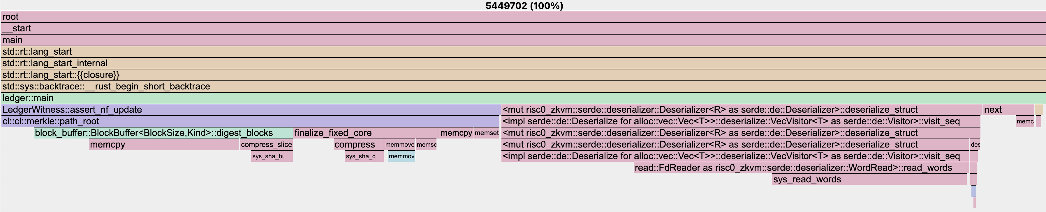
• SMT (2^256 depth):

• IMT (2^64 depth):

• Frontier-Based IMT:

Ledger Update

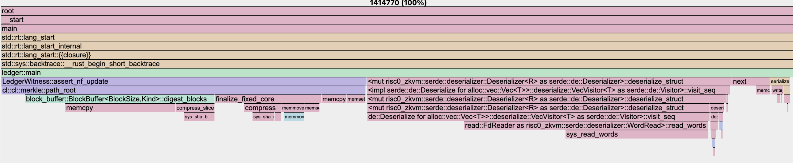
• SMT (2^256 depth): Approximately 5.4M million cycles were required for the addition of 4 nullifiers.

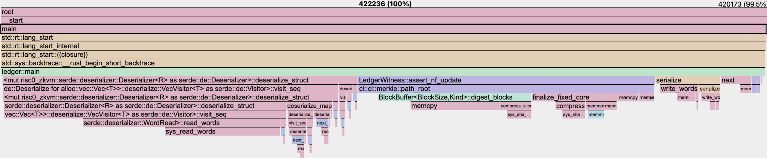
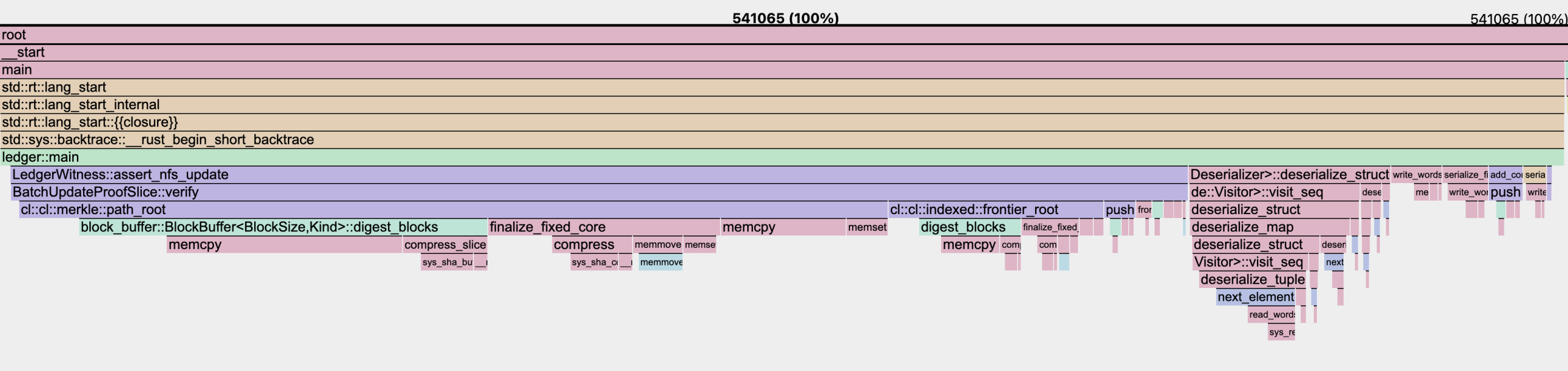
• Frontier-Based IMT: The same proof operation required 540,000 cycles (almost perfectly 10x, yay) for 4 nullifiers, indicating a substantial improvement. (An additional non-IMT-specific optimization for serialization was used as well)

Annex A

The root of a Merkle tree from its frontier can be computed as follows:

fn frontier_root(roots: &[Root]) -> [u8; 32] {
    if roots.is_empty() {
        return EMPTY_ROOTS[0];  // Empty root for a 0-depth tree.
    }
    let mut root = EMPTY_ROOTS[0];
    let mut depth = 1;
    for last in roots.iter().rev() {
        while depth < last.height {
            root = merkle::node(root, EMPTY_ROOTS[depth as usize - 1]);
            depth += 1;
        }
        root = merkle::node(last.root, root);
        depth += 1;
    }
    root
}

Since the frontier nodes represent sorted complete subtrees of decreasing height, the first frontier node already represents the left subtree of the full tree. We only need to obtain the right subtree and hash them together to get the tree root. We can recursively apply this reasoning to get all the intermediate roots, using precomputed empty subtree roots when needed.

[marvin.jones]

Very interesting.

For sparse Merkle trees, it is possible to reduce the proof size of non-membership proofs. Specifically, by storing the root hash of ‘empty’ trees for a variety of sizes, these hashes can be used to shorten the non-membership proof. This requires additional complexity to implement, but could address some of the communication complexity.

However, it seems the SMT and IMT both have scalability issues in terms of nullifiers getting too large. Polygon has an interesting proposal for nullifier windows that aims to address this. Though, it has a lot of drawbacks that affect users. But if something like this could be adapted to IMT, then the benefits of IMT can be maintained long-term.