Analysis of Failures in Mix Networks

[kd14]

Introduction

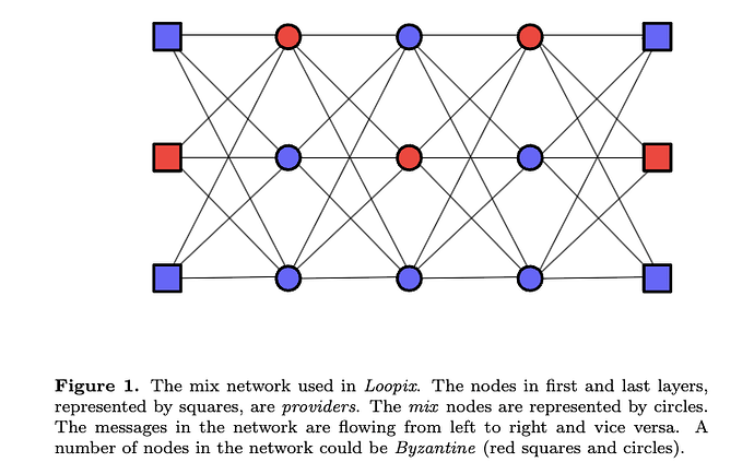
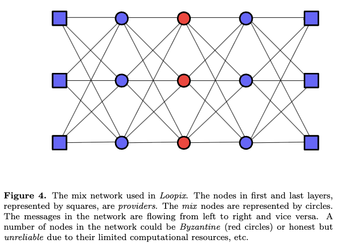
We consider anonymous communication system which uses a layered network of mix nodes, i.e. the mix network. We assume that nodes are used in the mix network are sampled from N nodes of a network where M nodes are adversarial. Presence of adversarial nodes in a communication path of the mix network can cause anonymity or communication failure. For anonymity failure to occur in a communication path all mix nodes on this path have to be adversarial and such path is compromised. In a mix network with L layers naive reasoning (e.g. see the article) gives (M/N)^L for the fraction of compromised paths. The latter is correct for a mix network of infinite width, but when the width is finite the fraction of compromised paths can be significantly larger than (M/N)^L. In this document we study statistical properties of the fraction compromised paths. Result of this work allows us to estimate the probability that the fraction of compromised paths is greater than some threshold. The latter can be used to optimise layered mix networks.

Assumptions

• To construct the mixnet we sample n nodes (without replacement) from the population of N nodes.

• At most M , where M<N, nodes in the population are adversarial.

• The number of adversarial nodes m in the mixnet is random number from the hypergeometric probability distribution P\left(m\vert N,n,M\right)=\frac{{n\choose m}{N-n\choose M-m}}{{N\choose M}}

• We have L layers constructed from n=\sum_{\mu=1}^L n_\mu nodes, where n_\mu is the number of nodes in the layer \mu.

• The probability that the number of adversarial nodes in layer 1 is m_1, in layer 2 is m_2, etc., is given by the multivariate hypergeometric distribution P\left(m_{1},\ldots, m_{L}\vert n_{1},\ldots,n_{L}; m\right)=\frac{\delta_{m;\sum_{\mu=1}^L m_{\mu}}\prod_{\mu=1}^L {n_\mu\choose m_\mu}}{{n\choose m}},

  where \delta_{x;y} in above is the Kronecker delta function.

• From above follows the joint probability distribution P\left(m_{1},\ldots, m_{L}\vert n_{1},\ldots,n_{L}\right)=\sum_{m=0}^nP\left(m_{1},\ldots, m_{L}\vert n_{1},\ldots,n_{L}; m\right)P\left(m\vert N,n,M\right)

Failures

• Anonymity failure occurs in the mix network when at least one adversarial node is present in each layer thus allowing to form a path of compromised nodes.
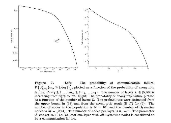
• The probability of anonymity failure is given by P\left(m_{1}\geq1,\ldots, m_{L}\geq1\vert n_{1},\ldots,n_{L}\right)

• Communication failure occurs in the mix network when the number of adversarial nodes is greater than some fraction A of nodes in at least one layer. A layer with all (or a large number) of adversarial (or honest but with limited resources) nodes could prevent (or considerably slow down) communication between users.
• We are interested in probability of the event \cup_{\mu=1}^L\{m_\mu\geq \lfloor An_\mu\rfloor\}, i.e. in at least one layer of the mix network the number of adversarial nodes is greater than some fraction A\in(0,1] of nodes in that layer.
• The probability of communication failure is given by P\left(\cup_{\mu=1}^L\{m_\mu\geq \lfloor An_\mu\rfloor\}\right)=1\!-\!P\left(m_1\!<\! \lfloor An_1\rfloor,\ldots,m_L\!<\! \lfloor An_L\rfloor\right),

• In the mix network of a fixed width the probability of anonymity failure and communication failure is, respectively, decreasing and increasing as the number of layers L is increasing.

Fraction of compromised paths

• The fraction of compromised paths \alpha\left(\{m_\mu\}\right) in the mix network of n=\sum_{\mu=1}^L n_\mu nodes distributed into L layers, where n_\mu is the number of nodes in layer \mu, is given by

\alpha\left(\{m_\mu\}\right)= \prod_{\mu=1}^L \frac{m_\mu}{n_\mu},

where m_\mu is the number of adversarial nodes in layer \mu and m=\sum_{\mu=1}^L m_\mu.

• For the mixnet of size n sampled from N nodes, where M<N nodes are adversarial, the average of the fraction of compromised paths \alpha\left(\{m_\mu\}\right) is expected to be (M/N)^L, where L is the number of layers, when the width n/L of the mixnet is very large.
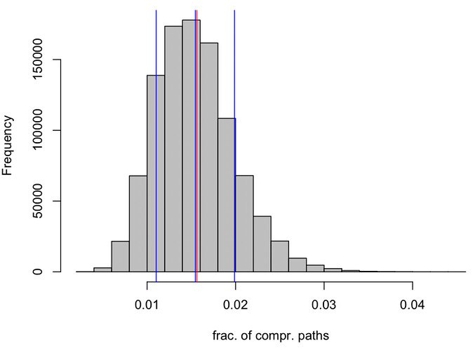
• We show that if assume large N then for large n, i.e. we first take N to infinity then n, the average of the random variable \alpha\left(\{m_\mu\}\right) is not (M/N)^L but it converges to the latter when the width n/L becomes infinite. Furthermore, in this limit the variance of \alpha vanishes and hence the fraction of compromised paths is exactly (M/N)^L.
• For the finite width n/L the fraction of compromised paths \alpha\left(\{m_\mu\}\right) can significantly deviate from (M/N)^L as can be seen in the following histogram

• We considered the probability that the fraction of compromised paths \alpha\left(\{m_\mu\}\right) belongs to the interval [\alpha_0, \alpha_1], where \alpha_0=a_0^L and \alpha_1=a_1^L. The lower bound on this probability can be obtained by assuming that fraction of adversarial nodes, P, in each layer of the mixnet is such that a_0\leq P\leq a_1. We use asymptotic approach to estimate the lower bound for large mixnet size n and below we compare this estimate with the same probability obtained in simulations.

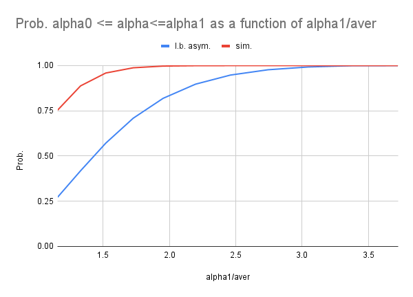
• Above suggests that the fraction of compromised paths can significantly deviate from the average (M/N)^L which assumes infinite mixnet width n/L.
• The probability P(\alpha_0\leq\alpha\left(\{m_\mu\}\right)\leq\alpha_1) can be used to obtain the probability 1-P(\alpha_0\leq\alpha\left(\{m_\mu\}\right)\leq\alpha_1) that the fraction of compromised paths \alpha\left(\{m_\mu\}\right) doesn’t belong to the interval [\alpha_0,\alpha_1].

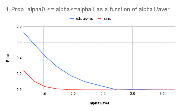
• For M/N=1/2 and L=3 the infinite width approximation gives (M/N)^L=1/8 fraction of compromised paths (this is example considered in the white paper Nym ) but asymptotic lower bound gives that fraction of compromised paths can be as high as 0.274625 (approx. 2.2 times greater than 1/8). The latter is verified in simulations.
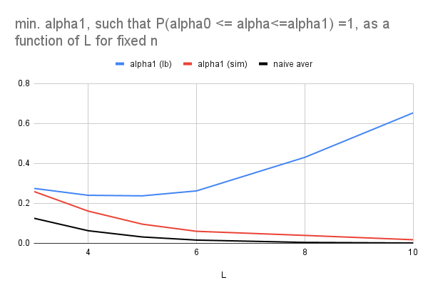
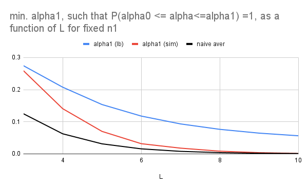
• For a given number of nodes n, sampled from N nodes, number of layers L and expected fraction of adversarial nodes M/N, the minimum of \alpha_1, \alpha_1^*, such that probability P(\alpha_0\leq\alpha\left(\{m_\mu\}\right)\leq\alpha_1)=1, i.e. \alpha_1^*=\mathrm{arg}\!\min_{\alpha_1}[P\left(\alpha_0\leq\alpha\left(\{m_\mu\}\right)\leq\alpha_1\right)=1], is the maximum fraction of compromised paths.
• The function which computes \alpha_1^*, using lower bound or exactly, can be used to design a program which optimises number of layers given some threshold on the fraction of compromised paths which can be tolerated.
• Using the (asymptotic) lower bound to compute \alpha_1^* gives a very loose upper bound on the maximum fraction of compromised paths when size of the mixnet n is fixed and number of layers L is increasing.

• The (asymptotic) lower bound gives a much tighter upper bound on \alpha_1^* when number of nodes per layer n_1 is fixed and number of layers L is increasing.

Binomial approximation

• For n_\mu=n_1, i.e. each layer has the same number of nodes, and n_1 large the fraction of compromised paths, \alpha(\{m_\mu\})= \prod_{\mu=1}^L \frac{m_\mu}{n_\mu}, in the mix network of n=L n_1 nodes, where m nodes are adversarial, is random variable from the distribution \langle\delta\!\left(\alpha-\alpha\left(\{m_\mu\}\right)\right)\rangle_m = \sum_{m_1=0}^{n_1}\cdots\sum_{m_L=0}^{n_1}\left\{\prod_{\mu=1}^L\mathrm{P}(m_\mu\vert n_1,m/n)\right\}\,\delta\!\left(\alpha-\alpha\left(\{m_\mu\}\right)\right), where \mathrm{P}(m_\mu\vert n_1,m/n) is the binomial distribution with parameters n_1 and m/n. Here \delta(x) is the Dirac’s delta function.
• The interpretation of above result is that when the number of nodes per layer n_1 is large then the number of adversarial nodes in the layer 1, m_1, in the layer 2, m_2, etc. are independent random variables sampled from the binomial distribution with parameters n_1 and m/n, i.e. in each layer on average n_1m/n nodes are adversarial.
• Furthermore, in the mixnet of size n sampled from N nodes, where M nodes are adversarial, the fraction of the fraction of compromised paths \alpha(\{m_\mu\}) is random variable from the distribution \langle\delta\!\left(\alpha-\alpha\left(\{m_\mu\}\right)\right)\rangle =\sum_{m=0}^{n}\mathrm{P}\left(m\vert N,n,M\right)\langle\delta\!\left(\alpha-\alpha\left(\{m_\mu\}\right)\right)\rangle_m, where \mathrm{P}\left(m\vert N,n,M\right) is the hypergeometric distribution of the number of adversarial nodes m in the mixnet of size n sampled from N nodes.

Improvement of the lower bound

• The lower bound on P(\alpha_0\leq\alpha(\{m_\mu\})\leq\alpha_1) considered in the previous section can be quite loose when number of nodes per layer n_1 is small as can be seen in the plot
• To improve the bound we consider the probability \mathrm{P}\left(\prod_{\mu=1}^Lm_{\mu}\geq\alpha_1\prod_{\mu=1}^Ln_{\mu}\right), i.e. the probability that the fraction of compromised paths \prod_{\mu=1}^L \frac{m_\mu}{n_\mu} is greater (or equal) to some \alpha_1.
• For \lambda>0 we have the upper bound \mathrm{P}\left(\prod_{\mu=1}^Lm_{\mu}\geq\alpha_1\prod_{\mu=1}^Ln_{\mu}\right)\leq \frac{\left\langle\exp(\lambda\prod_{\mu=1}^Lm_{\mu})\right\rangle}{\exp(\lambda\alpha_1\prod_{\mu=1}^L n_{\mu})}
• Furthermore, using in above the (AM-GM) inequality \prod_{\mu=1}^Lm_{\mu}\leq (\sum_{\mu=1}^Lm_{\mu}/L)^L we obtain the upper bound \mathrm{P}\left(\prod_{\mu=1}^Lm_{\mu}\geq\alpha_1\prod_{\mu=1}^Ln_{\mu}\right)\leq \frac{\left\langle\exp(\lambda(\sum_{\mu=1}^Lm_{\mu}/L)^L)\right\rangle}{\exp(\lambda\alpha_1\prod_{\mu=1}^L n_{\mu})} which is easier to compute.
• However, using in above the binomial approximation leads to very loose upper bound which is less than 1 only when \alpha_1 is close to 1.

Optimisation of mixnets using asymptotic lower bound

• We consider the algorithm which uses the (asymptotic) lower bound on the probability P(\alpha_0\leq\alpha(\{m_\mu\})\leq\alpha_1) that fraction of compromised paths \alpha(\{m_\mu\}) belongs to the interval [\alpha_0,\alpha_1] to find optimal parameters of the mixnet.
• The algorithm takes the number of nodes in population N, assumed fraction of adversarial nodes P, number of nodes in a layer n_1, minimum number of layers L_0, maximum number of layers L_1 and maximum fraction of compromised paths which can be tolerated \alpha_{\max}.
• Using above input the algorithm outputs the number of layers L and the fraction of compromised paths \alpha(\{m_\mu\}), where \alpha(\{m_\mu\})\leq\alpha_{\max}, corresponding to the latter.
• The code which computes the lower bound is given below

def Prob_alpha_v1(m2, a0, a1):
    global n1, L

    n = n1 * L  # Number of nodes in the mixnet

    if m2 == L:
        return (math.comb(n1, 1) ** L) / math.comb(n, L)
    elif m2 == (a1 * n1):
        return (math.comb(n1, int(a1 * n1)) ** L) / math.comb(n, int(a1 * n1))
    else:
        P = m2 / n
        m0 = math.ceil(a0 * n1)
        m1 = math.floor(a1 * n1)

        if m0 == m1:
            return (math.comb(n1, m0) ** L) / math.comb(n, L * m0)
        else:
            MIN = minimize((P - (Aver_m(Q, m0, m1) / n1)) ** 2, Q=0..1)
            Q = eval(Q, MIN[2])

            if Q == 1.0:
                print("Q=1")

            Dist = P * math.log(P / Q) + (1 - P) * math.log((1 - P) / (1 - Q))
            psi = Dist + math.log(sum(math.comb(n1, m) * (Q ** m) * ((1 - Q) ** (n1 - m)) for m in range(m0, m1 + 1))) / n1

            Var_m = (sum(math.comb(n1, m) * m * m * (Q ** m) * ((1 - Q) ** (n1 - m)) for m in range(m0, m1 + 1)) /
                     sum(math.comb(n1, m) * (Q ** m) * ((1 - Q) ** (n1 - m)) for m in range(m0, m1 + 1))) - \
                    (Aver_m(Q, m0, m1) ** 2)

            Prob = math.sqrt(n1 * P * (1 - P) / Var_m) * math.exp(n * psi)

            return Prob

• Above uses the function

def Aver_m(Q, m0, m1):
    global n1
    SUM1 = sum(math.comb(n1, m) * m * (Q ** m) * ((1 - Q) ** (n1 - m)) for m in range(m0, m1 + 1))
    SUM2 = sum(math.comb(n1, m) * (Q ** m) * ((1 - Q) ** (n1 - m)) for m in range(m0, m1 + 1))
    return SUM1 / SUM2

Upper bound

• We consider scenario when n nodes are sampled (without replacement) from N nodes where M nodes are adversarial.

• The probability P(\alpha(\{m_\mu\})\geq\alpha_1), where \alpha(\{m_\mu\})= \prod_{\mu=1}^L \frac{m_\mu}{n_\mu} is the fraction of compromised paths in the mixnet with L layers, can be estimated by the upper bound

  \mathrm{P}\left(\alpha(\{m_\mu\})\geq\alpha_1\right) \leq \sum_{m=L}^{n}\mathrm{P}\left(m\vert N,n,M\right)\exp\left(\lambda(\alpha_1)\left[\left(\frac{m}{n}\right)^L-\alpha_1\right]\right)

  when \alpha_1>\frac{\sum_{m=L}^{n}\mathrm{P}\left(m\vert N,n,M\right)\left(\frac{m}{n}\right)^L}{\sum_{m=L}^{n}\mathrm{P}\left(m\vert N,n,M\right)} and n_\mu=n_1, i.e. the same number of nodes in each layer.

• Here \mathrm{P}\left(m\vert N,n,M\right) is hypergeometric distribution of the number of adversarial nodes m in the mixnet of size n sampled from the population of N nodes with M adversarial nodes.

• The \lambda(\alpha_1)>0 parameter in the upper bound minimises the function

  \phi(\lambda)= \sum_{m=L}^{n}\mathrm{P}\left(m\vert N,n,M\right)\exp\left(\lambda\left[\left(\frac{m}{n}\right)^L-\alpha_1\right]\right).

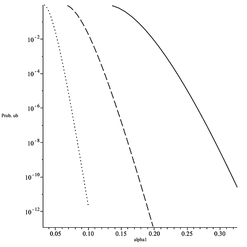
• The upper bound is tighter for larger \alpha_1 as can be seen in the figure below.

• For a give value of the upper bound on \mathrm{P}(\alpha(\{m_\mu\})\geq\alpha_1) and fixed width of the mixnet, the \alpha_1 is decreasing function of the number of layers L as can be seen in the figure below

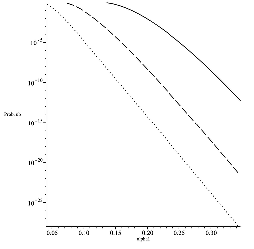
• For a give value of the upper bound on \mathrm{P}(\alpha(\{m_\mu\})\geq\alpha_1) and fixed size of the mixnet, n, the \alpha_1 is decreasing function of the number of layers L as can be seen in the figure below

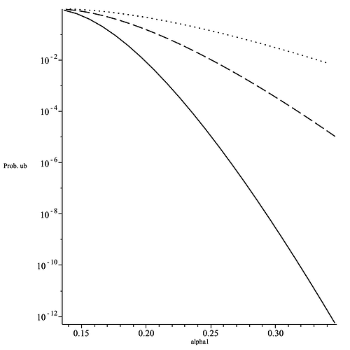
• For a give number of layers, L, the upper bound on \mathrm{P}(\alpha(\{m_\mu\})\geq\alpha_1) and is increasing with the decreasing mixnet width as can be seen in the figure below.

• In a scenario when all N nodes, where M nodes are adversarial, are used to construct the mixnet with L layers the fraction of compromised paths is at most (M/N)^L.
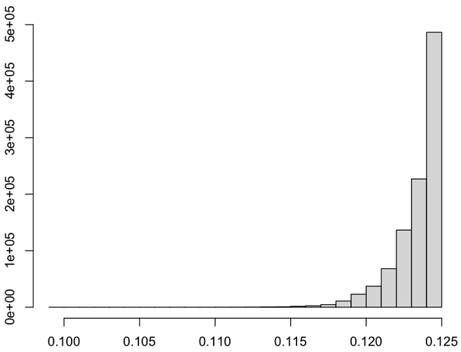
• The distribution of the fraction of compromised paths \alpha(\{m_\mu\}) has long left tail as can be seen in the figure below.

Using upper bound to optimise the mixnet

• We consider the algorithm which uses the upper bound on the probability \mathrm{P}(\alpha(\{m_\mu\})\geq\alpha_1) that fraction of compromised paths \alpha(\{m_\mu\}) is greater than \alpha_1 to find optimal parameters of the mixnet.
• The algorithm takes the number of nodes in population N, assumed fraction of adversarial nodes P, number of nodes in a layer n_1, minimum number of layers L_0, maximum number of layers L_1 and the probability \delta=\mathrm{P}(\alpha(\{m_\mu\})\geq\alpha_1) and maximum fraction of compromised paths which can be tolerated \alpha_{\max}.
• Using above input the algorithm outputs the number of layers L and the fraction of compromised paths \alpha(\{m_\mu\}), where \alpha(\{m_\mu\})\leq\alpha_{\max}, corresponding to the latter and given \delta.
• The code which computes the upper bound is given below

def Prob_ub(lambda_val, alpha1):
    global N, M, n, L, BINOM_N_M, AVER0
    
    if alpha1 <= AVER0:
        print("Increase alpha1!")
        return 0.0
    else:
        Z = BINOM_N_M * math.exp(lambda_val * alpha1)
        return sum(math.comb(n, m) * math.comb(N - n, M - m) * math.exp(lambda_val * (m / n)**L) for m in range(L, n + 1)) / Z

• In above for a given number of layers L the \mathsf{AVER0} for is computed by

def Aver0(L):
    global N, M, n1

    n = n1 * L
    SUM1 = sum(math.comb(n, m) * math.comb(N - n, M - m) * (m / n)**L for m in range(L, n + 1))
    SUM2 = sum(math.comb(n, m) * math.comb(N - n, M - m) for m in range(L, n + 1))

    return SUM1 / SUM2

• The BINOM_N_M is the binomial coefficient {N\choose M}.
• For a given alpha_1 the Prob_ub is minimised with respect to lambda_val to obtain the tightest possible bound.